Directional coupler on coupled RF lines. Analysis, general calculation formulas

Coupled RF transmission lines are used to create filters, combiners and dividers, directional couplers, VSWR meters, and so on. At high frequencies, such lines are most often created using microstrip technology and can be either symmetrical or asymmetrical, with a variety of space configurations. This article serves as a reference for our calculators dedicated to calculating such lines, as well as an example of using S-parameters.

To better understand the coupled line calculation method, let's use a real device—a directional coupler—as an example. This device consists of two coupled lines and has four ports.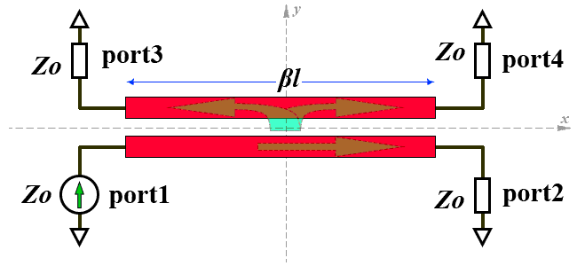
Since many radio amateurs have vector network analyzers, it's useful to perform an S-parameter analysis. Generally, a four-port device is characterized by 16 S-parameters. However, the directional coupler in our example has quadrature symmetry, meaning that if we draw an XY coordinate plane in our diagram, anything in one corner of this plane will be symmetrical to the other three. Simply put, both RF lines are exactly the same. In this case, the condition that several parameters of the S-scattering matrix are equal is satisfied, for example, S11 = S22 = S33 = S44. Then, it's sufficient to measure/calculate only four independent elements of the matrix, and the matrix itself will also look quite symmetrical:
The characteristic impedance of all ports is the same, and this value is called the “system impedance” of the device, Zo. In other words, the system impedance is the characteristic impedance of all its inputs/outputs.

The rather complex electromagnetic interaction of two RF lines, in which both forward and backward waves occur, can be reduced to two particular cases.

1. The RF lines are excited from ports 1 and 3 by two waves of equal amplitude and phase—in phase. This is called “even mode” excitation.
2. The lines are excited by two waves of equal amplitude and opposite phase—antiphase. This is called the “odd mode” of excitation.

The electromagnetic field configuration differs significantly in these two modes. The figure shows the configuration of the electric field lines:
It follows that at least the capacitance per unit length of each RF line is different in different modes, and therefore the characteristic impedances also differ. Therefore, concepts such as characteristic impedance for even excitation mode (Zeven) and for odd excitation mode (Zodd) are introduced. If the lines do not interact with each other, then Zeven = Zodd = Zo. When lines are coupled, Zeven and Zodd are always different, and the condition
Zeven > Zo > Zodd is always true. All these characteristic impedances are related by the following expression:

We are interested in the special case where the electrical length of the coupled RF lines is 90° or if the physical length is equal to a quarter of the wavelength. In this case, ctg(θ) = 0 and S31 is defined as follows: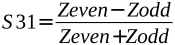
Analysis shows that for a quarter-wavelength line, S41 = 0 for an ideal directional coupler, meaning no wave enters the fourth port. In a real design, this free output must, of course, be loaded with an active resistance equal to the system impedance. This rule must also be observed when measuring the device with a vector analyzer. We connect the analyzer outputs to the ports whose parameters we are interested in, and always load the free ports with the system impedance.

An important parameter of a directional coupler is the coupling coefficient. The coupling coefficient of two coupled RF lines is uniquely determined by the ratio of the even and odd impedances: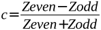
Since we're using S-parameters, let's base our discussion on them. It's then clear that the coupling coefficient (for our ideal example) is c = S31. The absolute value of the coupling coefficient is always less than one, which is quite logical and relates it to similar concepts from classical RLC-circuit theory. The coupling coefficient is usually expressed in decibel form: Cf = 20 log₁₀(c). In this case, the value of Cf is always negative, coinciding with the coupling coefficient expressed through its standard definition as the power ratio, and differing only in sign from “coupling loss”.

The forward wave proportion or forward transmission coefficient of an ideal directional coupler is determined by the following expression: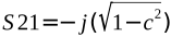
From the expression it follows that for c=1/√2 (or in decibel terms Cf=-3 dB), |S21| = |S31| and the wave is divided in half between outputs 3 and 2. Such a directional coupler is called a “three-decibel” coupler. “Insertion loss” is defined as follows: L = -20log₁₀(|S21|). The concept of “insertion loss” is completely identical to the concepts of “forward loss” or “operating loss” and always has a positive value. It is important to understand that in our example of an ideal directional coupler, the actual thermal losses in the line are not taken into account. The amount of power entering port 1 is the total that exits through ports 2 and 3. And the directional coupler parameters with the words “losses, attenuation” have no relation to actual thermal losses.

The phase of the wave at port 3 matches that of port 1, while the phase of port 2 lags by 90°. This lag is due to the propagation delay in the λ/4 line. The phase distribution is also evident from the formulas defining S31 and S21; simply recall the complex numbers plane looks like. These phase shifts must be taken into account when using a directional coupler, for example, as a combiner.

How to calculate a directional coupler on coupled lines? If we specify the system impedance and coupling coefficient, we can determine the even and odd impedances of the coupled lines:
The values ​​of even and odd impedance, in turn, depend on the cross-sectional dimensions of the coupled lines and the distance between them. Each type of such line has its own calculation method, as well as its own characteristics and limitations. For example, using microstrip lines with edge coupling, it is impossible to achieve a coupling coefficient greater than -10 dB, meaning that a 3-dB directional coupler based on them cannot be created; broadside coupling stripline must be used. Furthermore, the propagation constants for even and odd modes in microstrip coupled line differ, which presents an additional challenge.

Please note that we have to do with two two-wire coupled lines. The second conductor for each line is a common ground conductor or ground plane on the back of the PCB. However, in digital technology, such coupled lines are used as symmetrical or quasi-symmetrical differential pairs with a common reference ground. In this case, it is necessary to know the characteristic impedance of such a paired line for common-mode excitation Zcom and for differential excitation Zdif, which are determined by the following expressions:

Many people may have a reasonable question. Why, in our example, is port 3 coupled, while port 4 is isolated? Is this a mistake? After all, by theoretical logic, looking at the diagram, the “correct” direction should be the exact opposite. Moreover, most handbook and educational materials usually draw the diagram “correctly.” In reality, everything is much more complex, and tentative logic fails in this case. After all, the wave “jumping” from the main line 1-2 to the line 3-4 doesn't have any “inertia” that forces it to move exclusively toward port 4. It moves in both directions. All these waves, having “jumped” from different sections of the coupled line 1-2, add up (interfere) at the ports, taking into account their amplitude and phase. In the case of a line with a length of λ/4, they sum at port 3, and cancel each other out at port 4. But if the electrical length of the line is other (for example λ/2), the wave interference pattern changes, and ports 3 and 4 swap roles.

Related links:

• Power dividers and directional couplers;
• Coupled Line Couplers - Microwave Encyclopedia;
• Coupled-Line Couplers - The University of Kansas [PDF];
• Directional coupler 144 and 432 MHz - OK2KWW;
• 1296 MHz HOME MADE MICROSTRIP DIRECTIONAL COUPLERS - EA4NZ;