About RF transmission lines

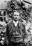
 To understand how you need to connect the feeder and the antenna, and why you need all these “baluns”, “matching networks” and other “muddles”, you can only understand the features of a radio signal propagation in long transmission lines. What are these lines - "long"? For the first time, telecommunications workers encountered "long lines" in 1866, when a communication cable was laid from Ireland to America, that is, long before the invention of radio. The length of the cable exceeded 2500 mi, and it was found that the telegraph signals transmitted through it expose to hard distortion, and it was almost impossible to receive and decode them. Understanding why this is happening was not for a long time. The outstanding self-taught English scientist Oliver Heaviside was able to clarify the issue.

In 1873, J.K.Maxwell's two-volume "Treatise on Electricity and Magnetism" came out of print. In this fundamental work, the world saw not only a coherent theory that brings together magnetic and electrical phenomena. The theory predicted the existence of electromagnetic waves and the finite speed of their propagation. The theory was accepted with hostility by the then scientific community. Do mention that the famous experiment of H.Hertz in 1887 had carried out just with the goal of refuting Maxwell's theory, but as a result, he experimentally confirmed the existence of electromagnetic waves. One of the few who immediately accepted Maxwell's theory was Heaviside. In 1885, his first article was published, where he showed that not only alternating current flows along telephone and telegraph lines, but an electromagnetic wave propagates along them with a finite speed. And if the line length is comparable to the wavelength, then the wave effects in the line must be taken into account. He, taking Maxwell's equations as a basis, created a mathematical model describing such a line in which reactance and resistance are "spread" along its total length. Therefore, another name for such a line is a line with distributed parameters. It is worth mentioning that the very concept of "inductance" was first introduced by Heaviside in his work on the theory of long transmission lines.

The equations describing the working of a long transmission line are still called "telegraph equations", since they appeared in the era of wire telegraph. In fact, telegraph equations are Ohm's and Kirchhoff's circuit laws in differential form. That is, the basic laws of the electrical circuit are also observed here, only one rule has been added - the interaction is not propagated instantly, but at a limited speed. And if for a low-frequency signal this fact was discovered only on a line thousands of kilometers long, then at 3G-4G frequencies a piece of coaxial cable a few centimeters long is already a "long" line described by the same telegraph equations.

From the analysis of telegraph equations it follows that two waves propagate in the line, one in the forward direction, and the other (reflected) in the opposite direction. These waves form an interference pattern in the line, called a standing wave. In the animation, we see two moving waves - direct and reflected, and a standing wave is shown with a thick line: As you see, at some sections of the line, the voltage may exceed the voltage of the source. This phenomenon was the reason that the first transatlantic cable was put into operation only from the fifth attempt due to insulation breakdowns for reasons unknown at that time. In a real line, the wave is reflected not only from the load, but also from the signal source and the interference pattern is looking much more complicated than this animation.

Well, we, dear anonymous, are dealing with relatively low signals and a breakdown of the feeder insulation does not threaten us, but it still does not hurt to know the main properties of the line. We will not delve into the theory and not consider the primary parameters of the line included in the telegraph equations - capacitance and inductance per unit length, and we will immediately move on to the secondary ones:

1. Characteristic impedance. It is important to understand that this is not an active resistance that gives rise to energy loss, but a parameter characterizing the properties of the TL when it interacts with an electromagnetic wave. Most feeders in radio engineering are classified as "low-loss transmission lines", this is when the reactance of the line is much higher than the active resistance. For such lines, the statement is true that its characteristic impedance depends only on its geometry (the ratio of the dimensions of the conductors) and the properties of the dielectric. Links to calculators of the characteristic impedance of some "long" lines can be seen at the end of the article.
   
2. Line input impedance. Impedance at line input terminals. Depends on the load impedance Z_load, characteristic impedance Z₀ as well as the length of the line l.β=2π/λ - phase constant. l=x₀-x - the length of the transmission line from the load point x₀=0. The input impedance of a line generally changes as its length changes:If the line is loaded with an active resistance equal to its characteristic impedance, then its input impedance at any length is equal to the characteristic impedance and is only active. In this case, there is no reflected wave in the line and all the energy goes to the load. This mode is the complete matching mode.
3. Reflection coefficient by voltage. The ratio of the amplitudes of the reflected and direct waves. 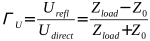Characterizes the degree of mismatching. Changes from zero (complete matching mode) to one (100% reflection). In the general case, the reflection coefficient is a complex (or a vector) value. In the theory of microwave devices, it is often replaced by the S11 parameter. S-parameters are described in more detail in another article.
4. Voltage standing wave ratio - VSWR is the ratio of the maximum voltage to the minimum voltage of the standing wave: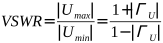It varies from unit with complete matching, to infinity with full reflection. For the line shown on the animation above Г_U=1, VSWR=∞.
5. Attenuation coefficient. In a real line, the energy of an electromagnetic wave is spent on heating the wires and the dielectric, so the wave is attenuated during propagation. Attenuation is measured in dB/m and increases with frequency.
6. Coefficient of shortening (velocity factor). The ratio of the wavelength in the line to the wavelength in free space. Any "long" line is a slowing-down structure and the wavelength in it is shorter than in vacuum, since the wave propagation velocity in the line is less than the free space light speed. For example, the propagation velocity in the mentioned transatlantic cable is 66% of the free space light speed, the same velocity in a common TV feeder with solid polyethylene inner insulation. In a balanced two-wire line, the slowdown is much less, only a few percent. This is true for the TEM wave, which requires a "two-wire" line to exist. But in the hollow wave-guides of the can or horn antennas, which are also lines with distributed parameters, the wavelength increases due to the same slowdown!

Of particular note are the cases of lines with lengths λ/4 and λ/2.

• λ/4 The input impedance of a quarter-wave segment is determined by the formula: With the short circuit at the load point (Z_l=0), there is infinite impedance at the input point! Such a short-circuited quarter-wave segment can be connected to another line, and it does not affect its work in any way. Such segments are called quarter-wave insulators. In addition, a quarter-wave segment is used to match the line with a load that has an impedance not equal to the characteristic impedance. Matching is done by selecting Z₀ in accordance with the above formula.A quarter-wave segment in its properties looks like a parallel LC-circuit, so another of its applications is a coaxial resonator.
• λ/2 In this case, the input impedance is always equal to the load impedance, regardless of the characteristic impedance. Such a segment is called a half-wave repeater and is quite often used in matching networks. In this case, the voltage phases at the ends of the half-wave segment are shifted by 180°.

This short article did not set itself the goal to look at the transmission lines theory in detail. There are important books about this. The main thing is to understand for yourself that the feeder is not just two wires connecting the antenna and the load, it is a complex circuit with distributed parameters that behaves "not quite adequately". A short-circuited segment of the feeder can have an infinitely large input resistance, a capacitance connected at one end of the feeder can turn into an inductance at the other, etc. There is only one reason for all this - the propagation speed of any interaction in our Universe is limited! This is what determines the complexity of understanding the working of matching networks, which we will view in the next article.

Related links:

• Coaxial characteristic impedance online calculator;
• Two-wire balanced TL characteristic impedance calculator;
• Twisted pair characteristic impedance calculator;